setwd("c:/ADP/data")
BlackFriday <- read.csv("BlackFriday.csv")
str(BlackFriday)
# 'data.frame': 537577 obs. of 12 variables:
# $ User_ID : int 1000001 1000001 1000001 1000001 1000002 1000003 1000004 1000004 1000004 1000005 ...
# $ Product_ID : chr "P00069042" "P00248942" "P00087842" "P00085442" ...
# $ Gender : chr "F" "F" "F" "F" ...
# $ Age : chr "0-17" "0-17" "0-17" "0-17" ...
# $ Occupation : int 10 10 10 10 16 15 7 7 7 20 ...
# $ City_Category : chr "A" "A" "A" "A" ...
# $ Stay_In_Current_City_Years: chr "2" "2" "2" "2" ...
# $ Marital_Status : int 0 0 0 0 0 0 1 1 1 1 ...
# $ Product_Category_1 : int 3 1 12 12 8 1 1 1 1 8 ...
# $ Product_Category_2 : int NA 6 NA 14 NA 2 8 15 16 NA ...
# $ Product_Category_3 : int NA 14 NA NA NA NA 17 NA NA NA ...
# $ Purchase : int 8370 15200 1422 1057 7969 15227 19215 15854 15686 7871 ...
# 모든 컬럼에 있는 NA 개수를 구해준다.
# product_Category_2, product_Category_3에 NA가 존재
colSums(is.na(BlackFriday))
# User_ID Product_ID Gender Age
# 0 0 0 0
# Occupation City_Category Stay_In_Current_City_Years Marital_Status
# 0 0 0 0
# Product_Category_1 Product_Category_2 Product_Category_3 Purchase
# 0 166986 373299 0
# 결측치 대체
# ifelse를 통해 결측치 NA값을 0으로 대체한다.
BlackFriday$Product_Category_2 <- ifelse(is.na(BlackFriday$Product_Category_2)==TRUE, 0, BlackFriday$Product_Category_2)
BlackFriday$Product_Category_3 <- ifelse(is.na(BlackFriday$Product_Category_3)==TRUE, 0, BlackFriday$Product_Category_3)
# summary 함수를 통해 확인한 결과 NA 값이 없음을 알 수 있다.
summary(BlackFriday)
# User_ID Product_ID Gender Age Occupation City_Category Stay_In_Current_City_Years Marital_Status Product_Category_1 Product_Category_2 Product_Category_3
# Min. :1000001 Length:537577 Length:537577 Length:537577 Min. : 0.000 Length:537577 Length:537577 Min. :0.0000 Min. : 1.000 Min. : 0.000 Min. : 0.000
# 1st Qu.:1001495 Class :character Class :character Class :character 1st Qu.: 2.000 Class :character Class :character 1st Qu.:0.0000 1st Qu.: 1.000 1st Qu.: 0.000 1st Qu.: 0.000
# Median :1003031 Mode :character Mode :character Mode :character Median : 7.000 Mode :character Mode :character Median :0.0000 Median : 5.000 Median : 5.000 Median : 0.000
# Mean :1002992 Mean : 8.083 Mean :0.4088 Mean : 5.296 Mean : 6.785 Mean : 3.872
# 3rd Qu.:1004417 3rd Qu.:14.000 3rd Qu.:1.0000 3rd Qu.: 8.000 3rd Qu.:14.000 3rd Qu.: 8.000
# Max. :1006040 Max. :20.000 Max. :1.0000 Max. :18.000 Max. :18.000 Max. :18.000
# Purchase
# Min. : 185
# 1st Qu.: 5866
# Median : 8062
# Mean : 9334
# 3rd Qu.:12073
# Max. :23961
# product_all 변수를 추가한다.
# 문제에 주어진 특정변수 데이터 타입을 확인한 뒤, 적절한 타입으로 변환한다.
BlackFriday<-transform(BlackFriday, product_all=Product_Category_1 + Product_Category_2 + Product_Category_3)
# 데이터 형태 변환
BlackFriday$User_ID<-as.character(BlackFriday$User_ID)
BlackFriday$Occupation<-as.factor(BlackFriday$Occupation)
BlackFriday$Marital_Status<-as.factor(BlackFriday$Marital_Status)
BlackFriday$Product_Category_1<-as.factor(BlackFriday$Product_Category_1)
BlackFriday$Product_Category_2<-as.factor(BlackFriday$Product_Category_2)
BlackFriday$Product_Category_3<-as.factor(BlackFriday$Product_Category_3)
str(BlackFriday)
# 'data.frame': 537577 obs. of 13 variables:
# $ User_ID : chr "1000001" "1000001" "1000001" "1000001" ...
# $ Product_ID : chr "P00069042" "P00248942" "P00087842" "P00085442" ...
# $ Gender : chr "F" "F" "F" "F" ...
# $ Age : chr "0-17" "0-17" "0-17" "0-17" ...
# $ Occupation : Factor w/ 21 levels "0","1","2","3",..: 11 11 11 11 17 16 8 8 8 21 ...
# $ City_Category : chr "A" "A" "A" "A" ...
# $ Stay_In_Current_City_Years: chr "2" "2" "2" "2" ...
# $ Marital_Status : Factor w/ 2 levels "0","1": 1 1 1 1 1 1 2 2 2 2 ...
# $ Product_Category_1 : Factor w/ 18 levels "1","2","3","4",..: 3 1 12 12 8 1 1 1 1 8 ...
# $ Product_Category_2 : Factor w/ 18 levels "0","2","3","4",..: 1 6 1 14 1 2 8 15 16 1 ...
# $ Product_Category_3 : Factor w/ 16 levels "0","3","4","5",..: 1 12 1 1 1 1 15 1 1 1 ...
# $ Purchase : int 8370 15200 1422 1057 7969 15227 19215 15854 15686 7871 ...
# $ product_all : num 3 21 12 26 8 3 26 16 17 8 ...
# 더미화를 위해 해당 변수에 대해 수치화한 후, caret 패키지의 dummyVars를 활용하여 더미화를 진행한다.
# 더미 변수화(Gender, Age, City_Category, Stay_In_Current_City_Years)
# 더미화를 위해 해당 변수 수치화
install.packages(c("caret","dplyr"))
library(caret)
library(dplyr)
# mutate 는 데이터프레임에 조건을 만족하는 새로운 열(변수)를 만들거나,
# 기존의 열을 조건에 맞게 변경할 때 사용합니다.
# 단, 새로 생성된 칼럼은 별도의 변수로 지정하거나 기존의 데이터에 덮어씌우지 않는 한 저장되지 않습니다.
BlackFriday_1 <- BlackFriday %>% mutate(Gender_binary = as.numeric(Gender),
Age_binary = as.numeric(Age),
City_Category_numeric = as.numeric(City_Category),
Stay_In_Current_City_Years_numeric = as.numeric(Stay_In_Current_City_Years))
dummy <- dummyVars("~ Gender + Age + City_Category + Stay_In_Current_City_Years", data = BlackFriday)
new_df <- data.frame(predict(dummy,newdata=BlackFriday))
BlackFriday_2<-cbind(BlackFriday,new_df)
str(BlackFriday_2)
# 'data.frame': 537577 obs. of 30 variables:
# $ User_ID : chr "1000001" "1000001" "1000001" "1000001" ...
# $ Product_ID : chr "P00069042" "P00248942" "P00087842" "P00085442" ...
# $ Gender : chr "F" "F" "F" "F" ...
# $ Age : chr "0-17" "0-17" "0-17" "0-17" ...
# $ Occupation : Factor w/ 21 levels "0","1","2","3",..: 11 11 11 11 17 16 8 8 8 21 ...
# $ City_Category : chr "A" "A" "A" "A" ...
# $ Stay_In_Current_City_Years : chr "2" "2" "2" "2" ...
# $ Marital_Status : Factor w/ 2 levels "0","1": 1 1 1 1 1 1 2 2 2 2 ...
# $ Product_Category_1 : Factor w/ 18 levels "1","2","3","4",..: 3 1 12 12 8 1 1 1 1 8 ...
# $ Product_Category_2 : Factor w/ 18 levels "0","2","3","4",..: 1 6 1 14 1 2 8 15 16 1 ...
# $ Product_Category_3 : Factor w/ 16 levels "0","3","4","5",..: 1 12 1 1 1 1 15 1 1 1 ...
# $ Purchase : int 8370 15200 1422 1057 7969 15227 19215 15854 15686 7871 ...
# $ product_all : num 3 21 12 26 8 3 26 16 17 8 ...
# $ GenderF : num 1 1 1 1 0 0 0 0 0 0 ...
# $ GenderM : num 0 0 0 0 1 1 1 1 1 1 ...
# $ Age0.17 : num 1 1 1 1 0 0 0 0 0 0 ...
# $ Age18.25 : num 0 0 0 0 0 0 0 0 0 0 ...
# $ Age26.35 : num 0 0 0 0 0 1 0 0 0 1 ...
# $ Age36.45 : num 0 0 0 0 0 0 0 0 0 0 ...
# $ Age46.50 : num 0 0 0 0 0 0 1 1 1 0 ...
# $ Age51.55 : num 0 0 0 0 0 0 0 0 0 0 ...
# $ Age55. : num 0 0 0 0 1 0 0 0 0 0 ...
# $ City_CategoryA : num 1 1 1 1 0 1 0 0 0 1 ...
# $ City_CategoryB : num 0 0 0 0 0 0 1 1 1 0 ...
# $ City_CategoryC : num 0 0 0 0 1 0 0 0 0 0 ...
# $ Stay_In_Current_City_Years0 : num 0 0 0 0 0 0 0 0 0 0 ...
# $ Stay_In_Current_City_Years1 : num 0 0 0 0 0 0 0 0 0 1 ...
# $ Stay_In_Current_City_Years2 : num 1 1 1 1 0 0 1 1 1 0 ...
# $ Stay_In_Current_City_Years3 : num 0 0 0 0 0 1 0 0 0 0 ...
# $ Stay_In_Current_City_Years4.: num 0 0 0 0 1 0 0 0 0 0 ...
# 특정변수 제외
BlackFriday_cluster <- BlackFriday_2 %>% select(-User_ID,
-Product_ID,
-Gender,
-Age,
-City_Category,
-Stay_In_Current_City_Years,
-product_all)
str(BlackFriday_cluster)
# 범주형 변수를 수치형 변수로 변환한다.
BlackFriday_cluster$Occupation<-as.numeric(BlackFriday_cluster$Occupation)
BlackFriday_cluster$Marital_Status<-as.numeric(BlackFriday_cluster$Marital_Status)
BlackFriday_cluster$Product_Category_1<-as.numeric(BlackFriday_cluster$Product_Category_1)
BlackFriday_cluster$Product_Category_2<-as.numeric(BlackFriday_cluster$Product_Category_2)
BlackFriday_cluster$Product_Category_3<-as.numeric(BlackFriday_cluster$Product_Category_3)
str(BlackFriday_cluster)
# 'data.frame': 537577 obs. of 27 variables:
# $ Occupation : num 11 11 11 11 17 16 8 8 8 21 ...
# $ Marital_Status : num 1 1 1 1 1 1 2 2 2 2 ...
# $ Product_Category_1 : num 3 1 12 12 8 1 1 1 1 8 ...
# $ Product_Category_2 : num 1 6 1 14 1 2 8 15 16 1 ...
# $ Product_Category_3 : num 1 12 1 1 1 1 15 1 1 1 ...
# $ Purchase : int 8370 15200 1422 1057 7969 15227 19215 15854 15686 7871 ...
# $ Gender_binary : num NA NA NA NA NA NA NA NA NA NA ...
# $ Age_binary : num NA NA NA NA NA NA NA NA NA NA ...
# $ City_Category_numeric : num NA NA NA NA NA NA NA NA NA NA ...
# $ Stay_In_Current_City_Years_numeric: num 2 2 2 2 NA 3 2 2 2 1 ...
# $ GenderF : num 1 1 1 1 0 0 0 0 0 0 ...
# $ GenderM : num 0 0 0 0 1 1 1 1 1 1 ...
# $ Age0.17 : num 1 1 1 1 0 0 0 0 0 0 ...
# $ Age18.25 : num 0 0 0 0 0 0 0 0 0 0 ...
# $ Age26.35 : num 0 0 0 0 0 1 0 0 0 1 ...
# $ Age36.45 : num 0 0 0 0 0 0 0 0 0 0 ...
# $ Age46.50 : num 0 0 0 0 0 0 1 1 1 0 ...
# $ Age51.55 : num 0 0 0 0 0 0 0 0 0 0 ...
# $ Age55. : num 0 0 0 0 1 0 0 0 0 0 ...
# $ City_CategoryA : num 1 1 1 1 0 1 0 0 0 1 ...
# $ City_CategoryB : num 0 0 0 0 0 0 1 1 1 0 ...
# $ City_CategoryC : num 0 0 0 0 1 0 0 0 0 0 ...
# $ Stay_In_Current_City_Years0 : num 0 0 0 0 0 0 0 0 0 0 ...
# $ Stay_In_Current_City_Years1 : num 0 0 0 0 0 0 0 0 0 1 ...
# $ Stay_In_Current_City_Years2 : num 1 1 1 1 0 0 1 1 1 0 ...
# $ Stay_In_Current_City_Years3 : num 0 0 0 0 0 1 0 0 0 0 ...
# $ Stay_In_Current_City_Years4. : num 0 0 0 0 1 0 0 0 0 0 ...
# kmeans 함수를 통해 군집분석을 수행한다.
set.seed(1234)
kmeans_BF<-kmeans(BlackFriday_cluster,3)
kmeans_BF
# K-means clustering with 3 clusters of sizes 119245, 252697, 165635
#
# Cluster means:
# Occupation Marital_Status Product_Category_1 Product_Category_2 Product_Category_3 Purchase GenderF GenderM
# 1 9.312164 1.406566 3.473278 7.398918 6.324022 17055.538 0.2006709 0.7993291
# 2 9.060527 1.411584 5.136032 6.955096 3.749827 9044.255 0.2566077 0.7433923
# 3 8.951363 1.406152 6.850804 7.091376 2.705219 4216.649 0.2621668 0.7378332
# Age0.17 Age18.25 Age26.35 Age36.45 Age46.50 Age51.55 Age55. City_CategoryA City_CategoryB City_CategoryC
# 1 0.02627364 0.1803262 0.3977022 0.2041092 0.08006206 0.07376410 0.03776259 0.2353893 0.4050652 0.3595455
# 2 0.02657728 0.1775526 0.3961108 0.2002952 0.08450832 0.07279469 0.04216117 0.2689545 0.4185883 0.3124572
# 3 0.02932955 0.1887524 0.4055302 0.1964923 0.08225315 0.06295167 0.03469074 0.2934464 0.4371962 0.2693573
# Stay_In_Current_City_Years0 Stay_In_Current_City_Years1 Stay_In_Current_City_Years2 Stay_In_Current_City_Years3
# 1 0.1307225 0.3494822 0.1906914 0.1750094
# 2 0.1364401 0.3514090 0.1841890 0.1735834
# 3 0.1368008 0.3545024 0.1821837 0.1725420
# Stay_In_Current_City_Years4.
# 1 0.1540945
# 2 0.1543786
# 3 0.1539711
#
# Clustering vector:
# 1 2 3 4 5 6 7 8 9 10 11 12 13 14 15 16 17 18 19 20 21 22 23 24
# 2 1 3 3 2 1 1 1 1 2 3 3 3 1 3 3 1 2 2 1 2 2 2 3
# 25 26 27 28 29 30 31 32 33 34 35 36 37 38 39 40 41 42 43 44 45 46 47 48
# 2 1 3 2 3 1 2 3 2 2 3 2 2 2 1 1 2 1 2 1 2 2 2 3
# 49 50 51 52 53 54 55 56 57 58 59 60 61 62 63 64 65 66 67 68 69 70 71 72
# 1 2 1 2 3 1 2 3 1 3 2 3 3 3 3 2 2 2 2 1 2 1 3 2
# 73 74 75 76 77 78 79 80 81 82 83 84 85 86 87 88 89 90 91 92 93 94 95 96
# 3 1 1 1 1 1 1 1 3 2 3 2 3 2 1 2 1 2 2 3 3 2 2 3
# 97 98 99 100 101 102 103 104 105 106 107 108 109 110 111 112 113 114 115 116 117 118 119 120
# 3 3 2 2 2 2 1 2 2 3 2 3 3 2 3 2 1 2 3 1 2 1 1 1
# 121 122 123 124 125 126 127 128 129 130 131 132 133 134 135 136 137 138 139 140 141 142 143 144
# 2 3 3 2 3 2 1 1 1 1 3 3 3 3 3 2 2 3 3 3 1 3 2 2
# 145 146 147 148 149 150 151 152 153 154 155 156 157 158 159 160 161 162 163 164 165 166 167 168
# 2 1 1 3 2 2 2 3 1 2 1 2 2 3 2 2 3 2 3 2 2 1 3 3
# 169 170 171 172 173 174 175 176 177 178 179 180 181 182 183 184 185 186 187 188 189 190 191 192
# 1 3 3 2 3 3 2 3 3 2 3 2 2 2 3 3 1 2 2 2 2 3 3 3
# 193 194 195 196 197 198 199 200 201 202 203 204 205 206 207 208 209 210 211 212 213 214 215 216
# 3 3 3 2 3 2 1 2 2 2 2 2 1 2 2 2 1 2 3 2 1 1 2 1
# 217 218 219 220 221 222 223 224 225 226 227 228 229 230 231 232 233 234 235 236 237 238 239 240
# 1 1 1 2 2 1 3 3 1 3 2 2 1 2 3 3 3 2 1 1 2 2 3 2
# 241 242 243 244 245 246 247 248 249 250 251 252 253 254 255 256 257 258 259 260 261 262 263 264
# 2 1 3 1 3 2 2 3 2 3 3 3 3 3 3 3 3 2 2 3 3 2 2 2
# 265 266 267 268 269 270 271 272 273 274 275 276 277 278 279 280 281 282 283 284 285 286 287 288
# 3 3 1 2 3 2 1 2 3 1 2 2 2 3 3 3 1 2 1 2 2 2 3 3
# 289 290 291 292 293 294 295 296 297 298 299 300 301 302 303 304 305 306 307 308 309 310 311 312
# 3 3 3 2 2 1 1 2 2 3 3 1 1 1 1 2 3 2 1 2 1 1 1 3
# 313 314 315 316 317 318 319 320 321 322 323 324 325 326 327 328 329 330 331 332 333 334 335 336
# 2 1 2 2 1 1 1 3 2 2 3 2 1 2 2 2 2 2 1 2 1 3 3 3
# 337 338 339 340 341 342 343 344 345 346 347 348 349 350 351 352 353 354 355 356 357 358 359 360
# 2 2 3 3 2 3 1 1 2 1 1 2 2 2 2 1 3 2 2 3 3 2 2 2
# 361 362 363 364 365 366 367 368 369 370 371 372 373 374 375 376 377 378 379 380 381 382 383 384
# 2 3 2 3 3 3 3 2 2 2 3 3 1 3 2 1 1 2 1 1 2 2 2 2
# 385 386 387 388 389 390 391 392 393 394 395 396 397 398 399 400 401 402 403 404 405 406 407 408
# 1 3 2 2 3 2 2 3 1 1 1 1 2 1 2 2 2 2 2 2 2 2 2 2
# 409 410 411 412 413 414 415 416 417 418 419 420 421 422 423 424 425 426 427 428 429 430 431 432
# 2 3 2 2 3 2 2 1 1 2 2 1 1 1 2 1 1 2 3 1 1 3 2 2
# 433 434 435 436 437 438 439 440 441 442 443 444 445 446 447 448 449 450 451 452 453 454 455 456
# 2 2 2 1 2 3 2 3 3 3 2 2 2 2 3 2 2 2 1 2 2 2 2 2
# 457 458 459 460 461 462 463 464 465 466 467 468 469 470 471 472 473 474 475 476 477 478 479 480
# 2 1 2 2 2 2 3 3 2 1 3 1 1 3 3 3 2 2 2 2 3 3 2 2
# 481 482 483 484 485 486 487 488 489 490 491 492 493 494 495 496 497 498 499 500 501 502 503 504
# 2 2 1 3 3 2 3 3 3 2 2 3 2 3 2 2 1 3 3 3 3 3 3 3
# 505 506 507 508 509 510 511 512 513 514 515 516 517 518 519 520 521 522 523 524 525 526 527 528
# 3 3 1 3 2 3 2 2 1 1 1 2 2 2 1 2 1 2 2 3 2 3 1 3
# 529 530 531 532 533 534 535 536 537 538 539 540 541 542 543 544 545 546 547 548 549 550 551 552
# 2 2 3 2 2 2 3 2 3 2 2 3 1 2 2 3 2 2 2 1 1 1 1 2
# 553 554 555 556 557 558 559 560 561 562 563 564 565 566 567 568 569 570 571 572 573 574 575 576
# 3 2 3 3 2 3 1 1 1 1 3 2 3 2 2 2 1 2 1 3 3 2 3 3
# 577 578 579 580 581 582 583 584 585 586 587 588 589 590 591 592 593 594 595 596 597 598 599 600
# 1 2 2 2 1 3 1 1 2 2 3 1 1 2 2 2 2 3 2 3 2 1 2 2
# 601 602 603 604 605 606 607 608 609 610 611 612 613 614 615 616 617 618 619 620 621 622 623 624
# 3 3 3 3 3 2 2 1 1 1 2 2 1 2 1 3 2 3 2 3 3 1 1 3
# 625 626 627 628 629 630 631 632 633 634 635 636 637 638 639 640 641 642 643 644 645 646 647 648
# 1 3 3 3 2 3 1 1 1 2 1 1 1 3 1 1 2 2 3 2 2 2 3 1
# 649 650 651 652 653 654 655 656 657 658 659 660 661 662 663 664 665 666 667 668 669 670 671 672
# 1 1 1 2 1 3 1 3 1 3 2 2 1 1 3 1 1 3 3 1 1 1 1 1
# 673 674 675 676 677 678 679 680 681 682 683 684 685 686 687 688 689 690 691 692 693 694 695 696
# 1 1 1 1 2 2 2 2 3 3 3 2 2 2 2 2 3 3 2 2 2 2 2 2
# 697 698 699 700 701 702 703 704 705 706 707 708 709 710 711 712 713 714 715 716 717 718 719 720
# 3 1 3 3 1 1 3 2 3 3 2 3 3 1 2 1 3 2 2 3 3 2 2 1
# 721 722 723 724 725 726 727 728 729 730 731 732 733 734 735 736 737 738 739 740 741 742 743 744
# 1 2 2 2 1 2 1 2 1 2 2 1 2 1 1 2 1 1 1 3 1 1 3 3
# 745 746 747 748 749 750 751 752 753 754 755 756 757 758 759 760 761 762 763 764 765 766 767 768
# 3 3 3 1 2 1 2 1 2 1 3 2 3 1 3 1 2 3 1 2 2 3 2 1
# 769 770 771 772 773 774 775 776 777 778 779 780 781 782 783 784 785 786 787 788 789 790 791 792
# 2 3 2 2 2 1 3 3 2 2 1 2 2 1 2 2 1 2 1 1 1 1 1 2
# 793 794 795 796 797 798 799 800 801 802 803 804 805 806 807 808 809 810 811 812 813 814 815 816
# 1 1 3 3 3 2 2 2 2 2 3 2 2 3 3 3 1 3 3 3 3 1 1 1
# 817 818 819 820 821 822 823 824 825 826 827 828 829 830 831 832 833 834 835 836 837 838 839 840
# 2 2 1 1 2 1 2 3 2 2 1 2 2 1 3 2 2 1 1 2 1 1 2 1
# 841 842 843 844 845 846 847 848 849 850 851 852 853 854 855 856 857 858 859 860 861 862 863 864
# 2 2 2 3 3 2 2 2 3 3 1 2 2 2 2 2 2 3 2 3 2 2 3 2
# 865 866 867 868 869 870 871 872 873 874 875 876 877 878 879 880 881 882 883 884 885 886 887 888
# 2 2 1 2 2 2 1 3 2 2 2 3 3 1 2 2 3 2 1 2 2 3 2 3
# 889 890 891 892 893 894 895 896 897 898 899 900 901 902 903 904 905 906 907 908 909 910 911 912
# 2 3 3 3 2 2 1 2 3 3 2 1 1 2 2 1 2 2 1 1 2 2 3 2
# 913 914 915 916 917 918 919 920 921 922 923 924 925 926 927 928 929 930 931 932 933 934 935 936
# 2 1 2 3 3 3 3 3 3 3 2 2 2 2 1 2 2 2 3 3 3 3 3 3
# 937 938 939 940 941 942 943 944 945 946 947 948 949 950 951 952 953 954 955 956 957 958 959 960
# 3 3 3 2 1 2 1 2 2 1 1 1 1 2 1 2 2 2 2 2 2 2 1 3
# 961 962 963 964 965 966 967 968 969 970 971 972 973 974 975 976 977 978 979 980 981 982 983 984
# 2 3 3 3 3 2 2 3 3 3 2 2 1 3 2 2 2 2 3 3 3 2 3 2
# 985 986 987 988 989 990 991 992 993 994 995 996 997 998 999 1000
# 2 2 2 3 2 1 3 1 1 1 3 1 1 1 1 3
# [ reached getOption("max.print") -- omitted 536577 entries ]
#
# Within cluster sum of squares by cluster:
# [1] 636141159429 810472759392 422633696404
# (between_SS / total_SS = 86.0 %)
#
# Available components:
#
# [1] "cluster" "centers" "totss" "withinss" "tot.withinss" "betweenss" "size" "iter"
# [9] "ifault"
# 해석
# kmeans 함수를 활용해 kmeans clustering을 수행했다. 군집의 수는 3개로 했으며, 각 군집에 119245,252697,165635개로 군집이 묶였다.
# between_SS / total_SS의 값이 86%로 나타나 군집이 잘되었다고 판단할 수 있다.
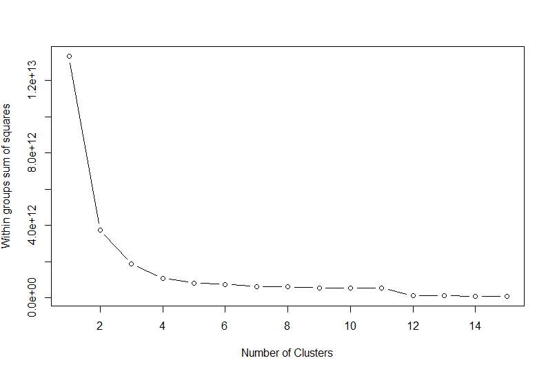
# Sum of square means 그래프를 통해 최적의 군집을 찾는다.
# Sum of square means 그래프로 최적의 군집 찾기
# 최소 군집 2개, 최대 군집 15개
wssplot <- function(data, nc=15, seed=1234){
wss <- (nrow(data) - 1) * sum(apply(data, 2, var)) # 열(column) 단위로 var 연산
for (i in 2:nc){
set.seed(seed)
wss[i] <- sum(kmeans(data, centers=i)$withinss)}
plot(1:nc, wss, type="b", xlab = "Number of Clusters",ylab = "Within groups sum of squares")}
wssplot(BlackFriday_cluster)
# 최적의 군집이 4개로 나타남
# 최적의 군집 개수로 군집의 개수를 변동하여 군집분석을 재수행한다.
# 군집의 개수를 4개로 하여 kmeans를 다시 실시
kmeans_BF_4 <- kmeans(BlackFriday_cluster, 4)
kmeans_BF_4

# K-means clustering with 4 clusters of sizes 109575, 89439, 106191, 232372
#
# Cluster means:
#   Occupation Marital_Status Product_Category_1 Product_Category_2 Product_Category_3  Purchase   GenderF   GenderM    Age0.17
# 1   9.326899       1.406042           3.460297           7.532576           6.425453 17380.202 0.1938763 0.8061237 0.02496920
# 2   8.939165       1.403594           7.168260           7.151131           3.032883  3000.617 0.2532452 0.7467548 0.03328526
# 3   9.143760       1.412031           4.351047           6.888559           5.017516 11276.081 0.2371199 0.7628801 0.02745995
# 4   8.994913       1.410622           5.871783           6.962633           2.761155  7089.676 0.2716463 0.7283537 0.02615634
# Age18.25  Age26.35  Age36.45   Age46.50   Age51.55     Age55. City_CategoryA City_CategoryB City_CategoryC
# 1 0.1785352 0.4000639 0.2037965 0.07990874 0.07438741 0.03833904      0.2349167      0.4041433      0.3609400
# 2 0.1978332 0.4060756 0.1910911 0.07978622 0.05884458 0.03308400      0.2981697      0.4345420      0.2672883
# 3 0.1781507 0.3917564 0.2028703 0.08342515 0.07384807 0.04248948      0.2610485      0.4180298      0.3209217
# 4 0.1784165 0.3999320 0.2002565 0.08510061 0.07041296 0.03972510      0.2776066      0.4258387      0.2965547
# Stay_In_Current_City_Years0 Stay_In_Current_City_Years1 Stay_In_Current_City_Years2 Stay_In_Current_City_Years3
# 1                   0.1304860                   0.3501072                   0.1901164                   0.1749395
# 2                   0.1377587                   0.3539731                   0.1828844                   0.1727099
# 3                   0.1356518                   0.3535987                   0.1836220                   0.1711350
# 4                   0.1364235                   0.3512514                   0.1840626                   0.1743885
# Stay_In_Current_City_Years4.
# 1                    0.1543509
# 2                    0.1526739
# 3                    0.1559925
# 4                    0.1538740
#
# Clustering vector:
#   1    2    3    4    5    6    7    8    9   10   11   12   13   14   15   16   17   18   19   20   21   22   23   24   25
# 4    1    2    2    4    1    1    1    1    4    4    2    4    1    4    2    3    4    3    1    4    3    3    4    3
# 26   27   28   29   30   31   32   33   34   35   36   37   38   39   40   41   42   43   44   45   46   47   48   49   50
# 1    4    4    4    1    4    4    4    3    4    4    3    4    1    1    4    1    4    1    3    3    3    4    1    4
# 51   52   53   54   55   56   57   58   59   60   61   62   63   64   65   66   67   68   69   70   71   72   73   74   75
# 1    4    4    1    3    4    1    4    3    4    2    2    4    4    3    3    4    1    4    1    2    3    2    1    1
# 76   77   78   79   80   81   82   83   84   85   86   87   88   89   90   91   92   93   94   95   96   97   98   99  100
# 1    1    1    1    3    2    4    4    4    4    4    1    3    1    4    3    2    2    4    4    2    2    2    3    4
# 101  102  103  104  105  106  107  108  109  110  111  112  113  114  115  116  117  118  119  120  121  122  123  124  125
# 3    4    1    3    4    4    4    4    2    4    2    3    1    4    4    1    3    1    1    1    3    4    2    4    2
# 126  127  128  129  130  131  132  133  134  135  136  137  138  139  140  141  142  143  144  145  146  147  148  149  150
# 4    1    1    1    1    2    2    4    4    4    3    4    4    4    4    1    2    4    4    3    1    1    2    4    4
# 151  152  153  154  155  156  157  158  159  160  161  162  163  164  165  166  167  168  169  170  171  172  173  174  175
# 4    2    1    4    1    3    3    2    4    4    4    3    2    4    4    1    4    4    1    4    4    4    2    4    4
# 176  177  178  179  180  181  182  183  184  185  186  187  188  189  190  191  192  193  194  195  196  197  198  199  200
# 2    2    4    2    4    4    4    4    4    1    4    3    4    4    4    4    4    2    4    4    3    2    4    1    4
# 201  202  203  204  205  206  207  208  209  210  211  212  213  214  215  216  217  218  219  220  221  222  223  224  225
# 4    4    4    4    1    4    4    4    1    3    2    4    1    1    3    1    1    1    1    4    3    1    4    4    1
# 226  227  228  229  230  231  232  233  234  235  236  237  238  239  240  241  242  243  244  245  246  247  248  249  250
# 4    4    3    1    3    2    2    4    4    1    1    4    4    2    4    3    3    2    1    2    3    4    2    4    2
# 251  252  253  254  255  256  257  258  259  260  261  262  263  264  265  266  267  268  269  270  271  272  273  274  275
# 2    2    2    2    2    4    2    4    4    2    2    4    4    4    2    2    1    3    4    4    1    3    4    1    3
# 276  277  278  279  280  281  282  283  284  285  286  287  288  289  290  291  292  293  294  295  296  297  298  299  300
# 4    4    2    4    4    1    4    1    3    3    3    2    2    2    2    2    3    3    3    1    3    4    4    4    1
# 301  302  303  304  305  306  307  308  309  310  311  312  313  314  315  316  317  318  319  320  321  322  323  324  325
# 1    1    1    4    2    4    1    3    1    1    1    4    3    1    3    3    3    1    1    2    4    3    2    3    1
# 326  327  328  329  330  331  332  333  334  335  336  337  338  339  340  341  342  343  344  345  346  347  348  349  350
# 3    4    3    4    4    1    4    1    4    4    4    3    3    2    2    3    2    1    1    3    3    1    4    4    4
# 351  352  353  354  355  356  357  358  359  360  361  362  363  364  365  366  367  368  369  370  371  372  373  374  375
# 4    1    4    4    3    4    2    4    4    3    4    4    3    4    2    2    2    4    4    4    2    2    1    4    3
# 376  377  378  379  380  381  382  383  384  385  386  387  388  389  390  391  392  393  394  395  396  397  398  399  400
# 1    1    3    1    1    4    4    3    4    1    4    4    3    4    4    4    2    1    3    1    1    3    1    4    4
# 401  402  403  404  405  406  407  408  409  410  411  412  413  414  415  416  417  418  419  420  421  422  423  424  425
# 4    3    4    3    4    3    3    4    4    2    3    4    4    4    4    1    1    3    4    1    1    1    3    3    3
# 426  427  428  429  430  431  432  433  434  435  436  437  438  439  440  441  442  443  444  445  446  447  448  449  450
# 3    4    1    1    2    3    3    3    4    4    1    3    4    4    4    4    2    4    4    4    4    2    4    4    4
# 451  452  453  454  455  456  457  458  459  460  461  462  463  464  465  466  467  468  469  470  471  472  473  474  475
# 1    3    3    4    3    4    4    1    4    4    4    3    4    2    3    1    4    1    1    2    2    2    3    4    4
# 476  477  478  479  480  481  482  483  484  485  486  487  488  489  490  491  492  493  494  495  496  497  498  499  500
# 4    2    4    4    4    4    4    1    2    4    3    4    2    2    3    4    4    4    4    4    4    3    2    2    2
# 501  502  503  504  505  506  507  508  509  510  511  512  513  514  515  516  517  518  519  520  521  522  523  524  525
# 4    4    4    2    2    2    1    2    3    4    4    3    3    1    1    4    3    3    1    4    1    3    3    2    4
# 526  527  528  529  530  531  532  533  534  535  536  537  538  539  540  541  542  543  544  545  546  547  548  549  550
# 2    1    2    4    4    4    4    4    3    4    4    2    3    4    4    1    3    4    2    3    4    3    1    1    1
# 551  552  553  554  555  556  557  558  559  560  561  562  563  564  565  566  567  568  569  570  571  572  573  574  575
# 1    3    2    4    2    2    4    2    1    1    1    1    4    4    2    3    4    4    1    3    1    2    4    3    2
# 576  577  578  579  580  581  582  583  584  585  586  587  588  589  590  591  592  593  594  595  596  597  598  599  600
# 2    1    4    4    4    1    4    3    1    3    3    2    1    1    4    3    4    3    4    4    2    4    1    4    3
# 601  602  603  604  605  606  607  608  609  610  611  612  613  614  615  616  617  618  619  620  621  622  623  624  625
# 4    2    2    2    4    4    3    1    1    1    4    3    1    3    1    4    4    4    4    2    4    1    1    2    1
# 626  627  628  629  630  631  632  633  634  635  636  637  638  639  640  641  642  643  644  645  646  647  648  649  650
# 2    2    4    3    2    1    1    1    3    1    1    1    4    1    1    4    4    2    3    4    4    2    1    1    1
# 651  652  653  654  655  656  657  658  659  660  661  662  663  664  665  666  667  668  669  670  671  672  673  674  675
# 1    3    1    2    1    4    1    4    4    4    1    1    4    1    1    2    2    1    1    1    1    1    1    1    1
# 676  677  678  679  680  681  682  683  684  685  686  687  688  689  690  691  692  693  694  695  696  697  698  699  700
# 1    4    4    4    4    4    4    4    4    4    4    4    4    4    2    4    4    3    4    4    4    2    1    2    2
# 701  702  703  704  705  706  707  708  709  710  711  712  713  714  715  716  717  718  719  720  721  722  723  724  725
# 1    1    2    4    2    2    4    2    2    1    4    1    4    4    4    4    4    4    3    1    1    3    3    4    1
# 726  727  728  729  730  731  732  733  734  735  736  737  738  739  740  741  742  743  744  745  746  747  748  749  750
# 4    1    3    1    4    4    1    3    1    1    4    1    1    1    2    1    1    2    2    2    4    2    1    3    1
# 751  752  753  754  755  756  757  758  759  760  761  762  763  764  765  766  767  768  769  770  771  772  773  774  775
# 4    1    4    1    4    3    2    1    4    1    3    2    1    4    3    2    4    1    4    2    3    3    4    1    2
# 776  777  778  779  780  781  782  783  784  785  786  787  788  789  790  791  792  793  794  795  796  797  798  799  800
# 4    4    4    1    4    4    1    3    4    1    3    1    1    1    1    1    3    1    1    2    2    2    4    4    4
# 801  802  803  804  805  806  807  808  809  810  811  812  813  814  815  816  817  818  819  820  821  822  823  824  825
# 4    4    4    3    4    2    4    4    1    4    4    4    4    1    1    1    3    4    1    1    3    1    4    4    4
# 826  827  828  829  830  831  832  833  834  835  836  837  838  839  840  841  842  843  844  845  846  847  848  849  850
# 3    1    4    4    1    4    4    4    1    1    4    3    1    4    1    3    3    4    4    4    4    3    4    2    4
# 851  852  853  854  855  856  857  858  859  860  861  862  863  864  865  866  867  868  869  870  871  872  873  874  875
# 1    4    4    4    4    4    3    4    4    4    4    4    4    4    4    4    1    4    4    4    1    4    4    4    4
# 876  877  878  879  880  881  882  883  884  885  886  887  888  889  890  891  892  893  894  895  896  897  898  899  900
# 4    2    1    3    3    4    4    1    4    4    4    3    4    4    2    4    4    3    3    3    3    2    4    4    1
# 901  902  903  904  905  906  907  908  909  910  911  912  913  914  915  916  917  918  919  920  921  922  923  924  925
# 1    4    3    1    4    3    3    1    3    4    4    4    3    1    4    2    2    2    2    2    2    2    4    3    3
# 926  927  928  929  930  931  932  933  934  935  936  937  938  939  940  941  942  943  944  945  946  947  948  949  950
# 3    1    4    3    4    2    2    2    2    2    2    2    2    4    3    1    4    1    3    3    1    1    1    1    4
# 951  952  953  954  955  956  957  958  959  960  961  962  963  964  965  966  967  968  969  970  971  972  973  974  975
# 1    4    3    3    4    4    3    3    1    2    3    4    4    4    4    4    4    4    2    4    3    4    1    2    4
# 976  977  978  979  980  981  982  983  984  985  986  987  988  989  990  991  992  993  994  995  996  997  998  999 1000
# 4    4    4    4    4    4    4    4    4    4    4    4    2    4    1    4    1    1    1    2    1    1    1    3    2
# [ reached getOption("max.print") -- omitted 536577 entries ]
#
# Within cluster sum of squares by cluster:
#   [1] 493145752071 124258692582 152898770978 314769926422
# (between_SS / total_SS =  91.9 %)
#
# Available components:
#
#   [1] "cluster"      "centers"      "totss"        "withinss"     "tot.withinss" "betweenss"    "size"         "iter"
# [9] "ifault"

# 해석

# 군집의 수를 4개로 하여 분석을 실시했으며, 각 군집에 106191, 232372, 109575, 89439개로 군집이 묶였다.
# berween_SS / total_SS의 값이 91.9%로 나타나 군집이 매우 잘되었다고 판단할 수 있다.


# 원본데이터에 분류된 결과를 각 행에 맞게 라벨링하여 clust 변수로 저장하여 csv파일로 출력한다,

kmeans_clust <- kmeans_BF_4$cluster
BlackFriday_full <- cbind(BlackFriday, clust=kmeans_clust)
str(BlackFriday_full)

# 'data.frame':	537577 obs. of  14 variables:
#   $ User_ID                   : chr  "1000001" "1000001" "1000001" "1000001" ...
# $ Product_ID                : chr  "P00069042" "P00248942" "P00087842" "P00085442" ...
# $ Gender                    : chr  "F" "F" "F" "F" ...
# $ Age                       : chr  "0-17" "0-17" "0-17" "0-17" ...
# $ Occupation                : Factor w/ 21 levels "0","1","2","3",..: 11 11 11 11 17 16 8 8 8 21 ...
# $ City_Category             : chr  "A" "A" "A" "A" ...
# $ Stay_In_Current_City_Years: chr  "2" "2" "2" "2" ...
# $ Marital_Status            : Factor w/ 2 levels "0","1": 1 1 1 1 1 1 2 2 2 2 ...
# $ Product_Category_1        : Factor w/ 18 levels "1","2","3","4",..: 3 1 12 12 8 1 1 1 1 8 ...
# $ Product_Category_2        : Factor w/ 18 levels "0","2","3","4",..: 1 6 1 14 1 2 8 15 16 1 ...
# $ Product_Category_3        : Factor w/ 16 levels "0","3","4","5",..: 1 12 1 1 1 1 15 1 1 1 ...
# $ Purchase                  : int  8370 15200 1422 1057 7969 15227 19215 15854 15686 7871 ...
# $ product_all               : num  3 21 12 26 8 3 26 16 17 8 ...
# $ clust                     : int  4 1 2 2 4 1 1 1 1 4 ...

# 군집의 개수를 4개로 하여 해당 cluster 분류를 열 결합하여 BlackFriday_full 데이터에 저장했다.
# 그리고 str 함수 구조를 파악해 clust 변수가 추가되었음을 확인하고 write.csv 함수로 해당 데이터를 csv 데이터로 출력했다.

# table 함수를 통해 군집 내 개수를 파악하고 xtabs 함수를 통해 군집별 특성을 파악한다,

table(BlackFriday_full$clust) # 군집내의 수는 2>3>1>4 순으로 많음
# 1      2      3      4
# 109575  89439 106191 232372

#Clust별 Gender 요약

xtabs(BlackFriday_full$clust ~ BlackFriday_full$Gender)

# F       M
# 394576 1141938

xtabs(~BlackFriday_full$clust + BlackFriday_full$Gender)

#                       BlackFriday_full$Gender
# BlackFriday_full$clust      F      M
#                       1  21244  88331
#                       2  22650  66789
#                       3  25180  81011
#                       4  63123 169249

# 해석

# 먼저 clust 개수를 파악하기 위해 table 함수를 사용했다. 2>3>1>4번 군집 순으로 군집이 묶였음을 알 수 있다.
# clust별 Gender를 요약할 때, xtabs 함수를 활용했다. 전체의 성비를 확인한 결과, Female이 3094576이고
# Male이 1141938로 Male이 약 3배 이상 많음을 파악할 수 있다. clust별 Gender를 확인한 결과 모든 clust에서
# Male의 숫자가 높았으며, 비율의 차이가 가장 많이 나는 군집은 3번 군집으로 나타났다.