통계분석 (사용 데이터 : Carseats)
# Urban 변수에 따른 Sales의 차이가 있는지를 통계적으로 검증하기 위한 통계분석을 수행하고,
# 결과를 해석하시오. (데이터는 정규성을 만족한다고 가정하고 유의수준 0.05하에서 검정)
## 데이터 불러오기
install.packages("ISLR")
library(ISLR)
data(Carseats)
car <- Carseats
str(car)
# 'data.frame': 400 obs. of 11 variables:
# $ Sales : num 9.5 11.22 10.06 7.4 4.15 ...
# $ CompPrice : num 138 111 113 117 141 124 115 136 132 132 ...
# $ Income : num 73 48 35 100 64 113 105 81 110 113 ...
# $ Advertising: num 11 16 10 4 3 13 0 15 0 0 ...
# $ Population : num 276 260 269 466 340 501 45 425 108 131 ...
# $ Price : num 120 83 80 97 128 72 108 120 124 124 ...
# $ ShelveLoc : Factor w/ 3 levels "Bad","Good","Medium": 1 2 3 3 1 1 3 2 3 3 ...
# $ Age : num 42 65 59 55 38 78 71 67 76 76 ...
# $ Education : num 17 10 12 14 13 16 15 10 10 17 ...
# $ Urban : Factor w/ 2 levels "No","Yes": 2 2 2 2 2 1 2 2 1 1 ...
# $ US : Factor w/ 2 levels "No","Yes": 2 2 2 2 1 2 1 2 1 2 ...
head(car)
# Sales CompPrice Income Advertising Population Price ShelveLoc Age Education Urban US
# 1 9.50 138 73 11 276 120 Bad 42 17 Yes Yes
# 2 11.22 111 48 16 260 83 Good 65 10 Yes Yes
# 3 10.06 113 35 10 269 80 Medium 59 12 Yes Yes
# 4 7.40 117 100 4 466 97 Medium 55 14 Yes Yes
# 5 4.15 141 64 3 340 128 Bad 38 13 Yes No
# 6 10.81 124 113 13 501 72 Bad 78 16 No Yes
## NA 값이 존재하는지 확인
sum(is.na(car))
# [1] 0
# Urban 변수에 따른 Sales의 차이를 통계적으로 검증하기 위한 독립표본 t-검정의 수행이 필요하다.
# 귀무가설 : 도시인지의 여부에 따른 판매량에는 차이가 없다.
# 대립가설 : 도시인지의 여부에 따른 판매량에는 차이가 있다.
# 독립표본 t-검정을 수행하기에 앞서, 두 집단 간의 데이터가 등분산성을 만족하는지 확인하기 위해
# 등분산 검정을 수행한다,
# 귀무가설 : 두 집단의 분산이 동일하다.
# 대립가설 : 두 집단의 분산이 동일하지 않다.
var.test(Sales~Urban, data=car, alternative="two.sided")
# F test to compare two variances
#
# data: Sales by Urban
# F = 0.9787, num df = 117, denom df = 281, p-value = 0.9072
# alternative hypothesis: true ratio of variances is not equal to 1
# 95 percent confidence interval:
# 0.7276615 1.3423111
# sample estimates:
# ratio of variances
# 0.9786966
# 해석
# 등분산 검정 결과 유의확률(p-value)이 0.9072로 유의수준 0.05보다 크기 때문에 귀무가설을 기각하지 않는다.
# 따라서 도시와 도시가 아닌 집단의 데이터는 등분산 가정을 만족한다고 볼 수 있다.
# 두 모집단이 등분산성 가정을 만족한다는 가정하에서 독립표본 t-검정을 수행한다.
t.test(Sales~Urban, data=car, alternative="two.sided", val.equal=TRUE)
# Welch Two Sample t-test
#
# data: Sales by Urban
# t = 0.30902, df = 221.57, p-value = 0.7576
# alternative hypothesis: true difference in means is not equal to 0
# 95 percent confidence interval:
# -0.5128302 0.7035658
# sample estimates:
# mean in group No mean in group Yes
# 7.563559 7.468191
# 해석
# 독립표본 t-검정 수행 결과, 검정통계량(t값)은 0.30765, 자유도(df)는 398, 유의확률 0.7576다.
# p-value가 유의수준 0.05보다 크기 때문에 귀무가설을 기각하지 않는다. 따라서 '도시지역과 도시가 아닌 지역간의
# 차 판매량에는 통계적으로 유의한 차이가 있다고 볼 수 없다.'는 결ㄹ론을 내릴 수 있다.
# Sales변수와 CompPrice, Income, Advertising, Population, Price, Age, Education 변수들 간에
# 피어슨 상관계수를 이용한 상관관계 분석을 수행하고 이를 해석하시오.
# Sales와 CompPrice 간의 상관분석
cor(car$Sales, car$CompPrice) # 피어슨 상관계수 산출
# [1] 0.06407873
cor.test(car$Sales, car$CompPrice) # 피어슨 상관계수 검정
# Pearson's product-moment correlation
#
# data: car$Sales and car$CompPrice
# t = 1.281, df = 398, p-value = 0.2009
# alternative hypothesis: true correlation is not equal to 0
# 95 percent confidence interval:
# -0.03418779 0.16111814
# sample estimates:
# cor
# 0.06407873
# 해석
# 상관계수는 약 0.064로 Sales와 CompPrice 간에는 거의 상관성이 존재하지 않는다고 볼 수 있다.
# p-value가 0.2009로 유의수준 0.05보다 크기 때문에 두 변수간의 상관관계는 통계적으로 유의하다고 볼 수 없다.
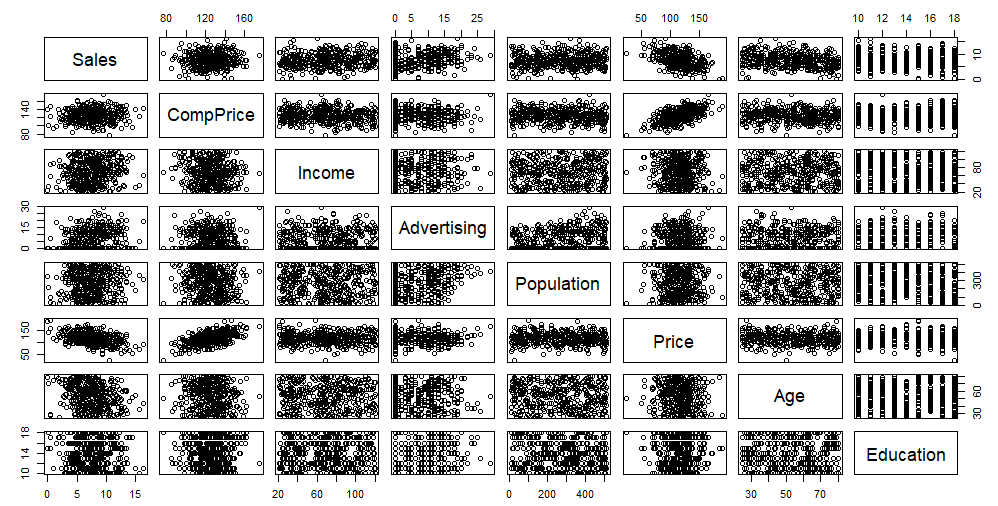
# 상관분석을 수행했던 변수들에 대해 상관계수 행렬을 생성하고 이를 시각화한다.
# 상관계수 행렬 생성 및 시각화
cor(car[,-c(7,10,11)])
# Sales CompPrice Income Advertising Population Price Age Education
# Sales 1.00000000 0.06407873 0.151950979 0.269506781 0.050470984 -0.44495073 -0.231815440 -0.051955242
# CompPrice 0.06407873 1.00000000 -0.080653423 -0.024198788 -0.094706516 0.58484777 -0.100238817 0.025197050
# Income 0.15195098 -0.08065342 1.000000000 0.058994706 -0.007876994 -0.05669820 -0.004670094 -0.056855422
# Advertising 0.26950678 -0.02419879 0.058994706 1.000000000 0.265652145 0.04453687 -0.004557497 -0.033594307
# Population 0.05047098 -0.09470652 -0.007876994 0.265652145 1.000000000 -0.01214362 -0.042663355 -0.106378231
# Price -0.44495073 0.58484777 -0.056698202 0.044536874 -0.012143620 1.00000000 -0.102176839 0.011746599
# Age -0.23181544 -0.10023882 -0.004670094 -0.004557497 -0.042663355 -0.10217684 1.000000000 0.006488032
# Education -0.05195524 0.02519705 -0.056855422 -0.033594307 -0.106378231 0.01174660 0.006488032 1.000000000
plot(car[,-c(7,10,11)])
# 종속변수를 Sales, 독립변수를 CompPrice, Income, Advertising, Population, Price, Age, Education으로 설정하고
# 후진제거법을 활용하여 회귀분석을 실시하고, 추정된 회귀식을 작성하시오.

# 후진제거법을 통한 변수선택 수행

step(lm(Sales~CompPrice+Income+Advertising+Population+Price+Age+Education, data=car), direction="backward")


# Start:  AIC=533.5
# Sales ~ CompPrice + Income + Advertising + Population + Price +
#   Age + Education
#
# Df Sum of Sq    RSS    AIC
# - Population   1      0.12 1458.7 531.53
# - Education    1      4.32 1462.9 532.68
# <none>                     1458.6 533.50
# - Income       1     51.03 1509.6 545.25
# - Age          1    208.48 1667.0 584.94
# - Advertising  1    278.65 1737.2 601.43
# - CompPrice    1    533.98 1992.5 656.28
# - Price        1   1247.94 2706.5 778.78
#
# Step:  AIC=531.53
# Sales ~ CompPrice + Income + Advertising + Price + Age + Education
#
# Df Sum of Sq    RSS    AIC
# - Education    1      4.21 1462.9 530.68
# <none>                     1458.7 531.53
# - Income       1     51.29 1510.0 543.35
# - Age          1    208.51 1667.2 582.97
# - Advertising  1    295.91 1754.6 603.41
# - CompPrice    1    540.75 1999.4 655.66
# - Price        1   1250.06 2708.7 777.11
#
# Step:  AIC=530.68
# Sales ~ CompPrice + Income + Advertising + Price + Age
#
# Df Sum of Sq    RSS    AIC
# <none>                     1462.9 530.68
# - Income       1     53.02 1515.9 542.92
# - Age          1    209.00 1671.9 582.10
# - Advertising  1    298.27 1761.2 602.91
# - CompPrice    1    539.21 2002.1 654.20
# - Price        1   1249.81 2712.7 775.70
#
# Call:
#   lm(formula = Sales ~ CompPrice + Income + Advertising + Price +
#        Age, data = car)
#
# Coefficients:
#   (Intercept)    CompPrice       Income  Advertising        Price          Age
# 7.10919      0.09390      0.01309      0.13061     -0.09254     -0.04497


# 해석

첫 번째 단계를 확인해보면 Population 변수가 모형에서 제거되었을 때 AIC값이 531.53으로 가장 작은 것을 확인할 수 있다.
따라서 첫 번째 단계에서 Population 변수가 모형에서 제거되었다.

두 번째 단계에서는 Education 변수가 제거되었을 때 AIC값이 가장 작아지기 때문에 Education 변수가 모형에서 제거되었다.

위와 같은 변수의 제거과정을 거쳐서 lm(formula = Sales~CompPrice + Income + Advertising + Price + Age,data=car)이라는 최종 모형이 결정되었다.
최종적으로 선택된 추정된 회귀식은 7.10919 + 0.09390*CompPrice + 0.01309*Income + 0.13061*Advertising - 0.09254*Price - 0.04497*Age이다.

# 앞서 진행한 후진제거법을 통해 선택된 변수들로 새로운 회귀모형을 생성한다.

# 변수 선택을 통해 도출된 회귀모형

cal.lm <- lm(Sales ~ CompPrice + Income + Advertising + Price + Age, data=car)
summary(cal.lm)

# Call:
#   lm(formula = Sales ~ CompPrice + Income + Advertising + Price +
#        Age, data = car)
#
# Residuals:
#   Min      1Q  Median      3Q     Max
# -4.9071 -1.3081 -0.1892  1.1495  4.6980
#
# Coefficients:
#   Estimate Std. Error t value Pr(>|t|)
# (Intercept)  7.109190   0.943940   7.531 3.46e-13 ***
#   CompPrice    0.093904   0.007792  12.051  < 2e-16 ***
#   Income       0.013092   0.003465   3.779 0.000182 ***
#   Advertising  0.130611   0.014572   8.963  < 2e-16 ***
#   Price       -0.092543   0.005044 -18.347  < 2e-16 ***
#   Age         -0.044971   0.005994  -7.503 4.20e-13 ***
#   ---
#   Signif. codes:  0 ‘***’ 0.001 ‘**’ 0.01 ‘*’ 0.05 ‘.’ 0.1 ‘ ’ 1
#
# Residual standard error: 1.927 on 394 degrees of freedom
# Multiple R-squared:  0.5403,	Adjusted R-squared:  0.5345
# F-statistic: 92.62 on 5 and 394 DF,  p-value: < 2.2e-16

# 해석

# 후진제거법을 이용한 변수 선택을 수행한 후 선택된 변수들로 회귀분석을 수행한 결과,
# 모든 변수들의 유의확률이 매우 작아 통계적으로 유의함을 확인할 수 있다. 하지만 모형의 결정계수는 0.5403,
# 수정된 결정계수는 0.5345로 추정된 다변량 회귀식은 전체 데이터의 변동의 약 53%를 설명하고 있어
# 다소 낮은 설명력을 가진다.
#
# 또한 회귀모형의 F통계량에 대한 p-value의 값은 0.05보다 작으므로 유의수준 0.05 하에서 모형이 통계적으로 유의한 것을 알 수 있다.