정형 데이터 마이닝 - 타이타닉
library(dplyr)
setwd("C:/ADP/data")
# 데이터 불러오기
titanic <- read.csv("titanic.csv")
summary(titanic)
# cabin, embarked의 "" -> NA 바꾸기
# embarked
# factor 형태로 변환
titanic$embarked <- as.factor(titanic$embarked)
levels(titanic$embarked)
# [1] "" "C" "Q" "S"
# "" -> NA 변환
levels(titanic$embarked)[1] <- NA
table(titanic$embarked,useNA = "always")
# C Q S <NA>
# 270 123 914 2
# cabin
titanic$cabin <- ifelse(titanic$cabin=="",NA,titanic$cabin)
table(titanic$cabin,useNA = "always")
summary(titanic)
# pclass survived name sex age
# Min. :1.000 Min. :0.000 Length:1309 Length:1309 Min. : 0.17
# 1st Qu.:2.000 1st Qu.:0.000 Class :character Class :character 1st Qu.:21.00
# Median :3.000 Median :0.000 Mode :character Mode :character Median :28.00
# Mean :2.295 Mean :0.382 Mean :29.88
# 3rd Qu.:3.000 3rd Qu.:1.000 3rd Qu.:39.00
# Max. :3.000 Max. :1.000 Max. :80.00
# NA's :263
# sibsp parch ticket fare
# Min. :0.0000 Min. :0.000 Length:1309 Min. : 0.000
# 1st Qu.:0.0000 1st Qu.:0.000 Class :character 1st Qu.: 7.896
# Median :0.0000 Median :0.000 Mode :character Median : 14.454
# Mean :0.4989 Mean :0.385 Mean : 33.295
# 3rd Qu.:1.0000 3rd Qu.:0.000 3rd Qu.: 31.275
# Max. :8.0000 Max. :9.000 Max. :512.329
# NA's :1
# cabin embarked
# Length:1309 C :270
# Class :character Q :123
# Mode :character S :914
# NA's: 2
# 변수의 데이터 타입 확인 뒤, 타입 변환
str(titanic)
# 'data.frame': 1309 obs. of 11 variables:
# $ pclass : int 1 1 1 1 1 1 1 1 1 1 ...
# $ survived: int 1 1 0 0 0 1 1 0 1 0 ...
# $ name : chr "Allen, Miss. Elisabeth Walton" "Allison, Master. Hudson Trevor" "Allison, Miss. Helen Loraine" "Allison, Mr. Hudson Joshua Creighton" ...
# $ sex : chr "female" "male" "female" "male" ...
# $ age : num 29 0.92 2 30 25 48 63 39 53 71 ...
# $ sibsp : int 0 1 1 1 1 0 1 0 2 0 ...
# $ parch : int 0 2 2 2 2 0 0 0 0 0 ...
# $ ticket : chr "24160" "113781" "113781" "113781" ...
# $ fare : num 211 152 152 152 152 ...
# $ cabin : chr "B5" "C22 C26" "C22 C26" "C22 C26" ...
# $ embarked: Factor w/ 3 levels "C","Q","S": 3 3 3 3 3 3 3 3 3 1 ...
# 변수의 데이터 타입 변환
titanic$pclass <- as.factor(titanic$pclass)
titanic$survived <- factor(titanic$survived,levels=c(0,1),labels=c("dead","survived"))
# 변환된 변수 확인
str(titanic)
# 결측치 대치
sum(!complete.cases(titanic))
# 모든 컬럼에 있는 NA 개수를 구해준다.
colSums(is.na(titanic))
# pclass survived name sex age sibsp parch ticket fare
# 0 0 0 0 263 0 0 0 1
# cabin embarked
# 1014 2
# 수치형 변수 결측치 중앙값 대체
titanic$age[is.na(titanic$age)] <- median(titanic$age, na.rm=TRUE)
sum(is.na(titanic$age))
titanic$fare[is.na(titanic$fare)] <- median(titanic$fare, na.rm = TRUE)
sum(is.na(titanic$fare))
# 변수형 변수 최빈값 대체
# 최빈값 함수
mode <- function(x){
return(names(sort(table(x), decreasing = T)[1] ) %>% as.character)
}
mode(titanic$embarked)
titanic$embarked[is.na(titanic$embarked)] <- mode(titanic$embarked)
sum(is.na(titanic$embarked))
titanic$cabin[is.na(titanic$cabin)] <- mode(titanic$cabin)
sum(is.na(titanic$cabin))
table(titanic$cabin)
# age의 범주를 나눔
titanic <- within(titanic,
{
age_band = integer(0)
age_band[age>=0 & age<10] = 0
age_band[age>=10 & age<20] = 1
age_band[age>=20 & age<30] = 2
age_band[age>=30 & age<40] = 3
age_band[age>=40 & age<50] = 4
age_band[age>=50 & age<60] = 5
age_band[age>=60 & age<70] = 6
age_band[age>=70 & age<80] = 7
age_band[age>=80 & age>90] = 8
})
titanic$age_band <- factor(titanic$age_band, levels=c(0,1,2,3,4,5,6,7,8),
labels=c("10세 미만","10대","20대","30대","40대","50대","60대","70대","80대"))
str(titanic)
# 데이터 분할
set.seed(12345)
idx <- sample(1:nrow(titanic),size=nrow(titanic)*0.7,replace=FALSE)
train_df <-titanic[idx,]
test_df<-titanic[-idx,]
nrow(train_df)
nrow(test_df)
# 모델링 하기 전 분석에 사용할 변수만 추출
train <- train_df[,c("pclass","survived","sex","sibsp","parch","fare","embarked")]
test <- test_df[,c("pclass","survived","sex","sibsp","parch","fare","embarked")]
str(train)
# 모델링 의사결정나무(깊이를 최대 5개까지, 최소 관측치는 15개 이상)
install.packages(c("rpart","rpart.plot"))
library(rpart)
library(rpart.plot)
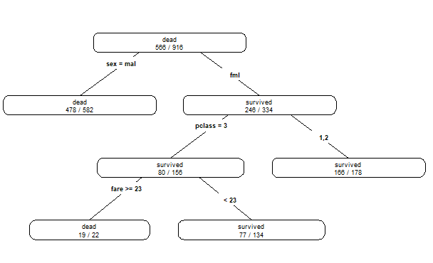
dt.model <- rpart(survived ~., method='class', data=train, control=rpart.control(maxdepth=4, minsplit=15))
dt.model
# n= 916
#
# node), split, n, loss, yval, (yprob)
# * denotes terminal node
#
# 1) root 916 350 dead (0.61790393 0.38209607)
# 2) sex=male 582 104 dead (0.82130584 0.17869416) *
# 3) sex=female 334 88 survived (0.26347305 0.73652695)
# 6) pclass=3 156 76 survived (0.48717949 0.51282051)
# 12) fare>=23.35 22 3 dead (0.86363636 0.13636364) *
# 13) fare< 23.35 134 57 survived (0.42537313 0.57462687) *
# 7) pclass=1,2 178 12 survived (0.06741573 0.93258427) *
prp(dt.model,type=4,extra=2)
pred <- predict(dt.model,test[,-2],type='prob')
write.csv(pred,"decisionTree predict.csv")

# 모델링 랜덤 포레스트
install.packages("randomForest")
library(randomForest)

rf.model <- randomForest(formula = survived~., data=train)
print(rf.model)

# Call:
#   randomForest(formula = survived ~ ., data = train)
# Type of random forest: classification
# Number of trees: 500
# No. of variables tried at each split: 2
#
# OOB estimate of  error rate: 20.52%
# Confusion matrix:
#   dead survived class.error
# dead      511       55  0.09717314
# survived  133      217  0.38000000

pred <- predict(rf.model,test[,-2],type="prob")
write.csv(pred,"randomForest predict.csv")

# 모델링 로지스틱 회귀분석
lg.model <- step(glm(survived~1, data=train, family="binomial"),direction="both",
                 scope=list(lower=~1, upper=~pclass+sex+sibsp+parch+fare+embarked))

summary(lg.model)


# Call:
#   glm(formula = survived ~ sex + pclass + embarked + sibsp, family = "binomial",
#       data = train)
#
# Deviance Residuals:
#   Min       1Q   Median       3Q      Max
# -2.2973  -0.6783  -0.4402   0.6838   2.3801
#
# Coefficients:
#   Estimate Std. Error z value Pr(>|z|)
# (Intercept)  2.56479    0.26026   9.855  < 2e-16 ***
#   sexmale     -2.68646    0.18501 -14.520  < 2e-16 ***
#   pclass2     -0.61090    0.25349  -2.410  0.01595 *
#   pclass3     -1.54394    0.21864  -7.062 1.64e-12 ***
#   embarkedQ   -0.31418    0.34788  -0.903  0.36646
# embarkedS   -0.61980    0.22001  -2.817  0.00485 **
#   sibsp       -0.16208    0.09883  -1.640  0.10100
# ---
#   Signif. codes:  0 ‘***’ 0.001 ‘**’ 0.01 ‘*’ 0.05 ‘.’ 0.1 ‘ ’ 1
#
# (Dispersion parameter for binomial family taken to be 1)
#
# Null deviance: 1218.43  on 915  degrees of freedom
# Residual deviance:  846.59  on 909  degrees of freedom
# AIC: 860.59
#
# Number of Fisher Scoring iterations: 4

pred <- predict(lg.model, test[,-2], type="response")
pred_df <- as.data.frame(pred)
pred_df$survived <- ifelse(pred_df$pred<=0.5,pred_df$survived<-"dead",pred_df$survived<-"survived")
write.csv(pred_df,"logistic regression predict.csv")

# 성과분석 - 의사결정나무
library(caret)
library(ROCR)
pred.dt<-predict(dt.model,test[,-2],type="class")
confusionMatrix(data=pred.dt, reference=test[,2],positive="survived")

# Confusion Matrix and Statistics
#
# Reference
# Prediction dead survived
# dead      215       57
# survived   28       93
#
# Accuracy : 0.7837
# 95% CI : (0.7397, 0.8234)
# No Information Rate : 0.6183
# P-Value [Acc > NIR] : 1.589e-12
#
# Kappa : 0.5242
#
# Mcnemar's Test P-Value : 0.002389
#
#             Sensitivity : 0.6200
#             Specificity : 0.8848
#          Pos Pred Value : 0.7686
#          Neg Pred Value : 0.7904
#              Prevalence : 0.3817
#          Detection Rate : 0.2366
#    Detection Prevalence : 0.3079
#       Balanced Accuracy : 0.7524
#
#        'Positive' Class : survived
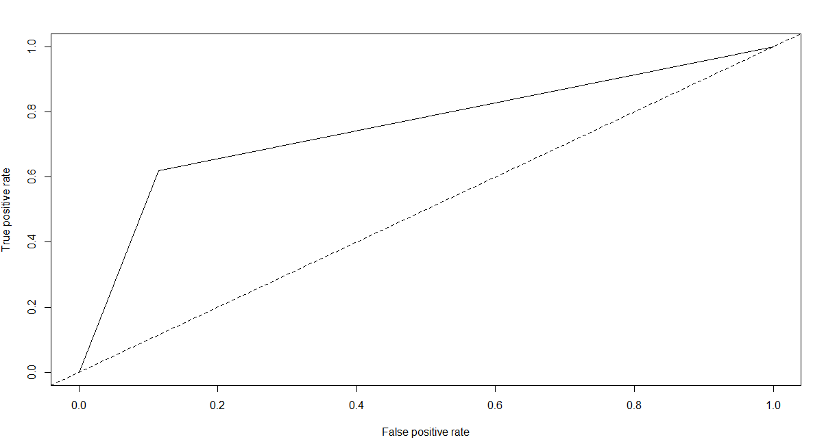
pred.dt.roc <- prediction(as.numeric(pred.dt),as.numeric(test[,2]))
plot(performance(pred.dt.roc,"tpr","fpr"))
abline(a=0,b=1,lty=2,col="black")
performance(pred.dt.roc,"auc")@y.values

# [[1]]
# [1] 0.7523868


# 성과분석 - 랜덤포레스트
pred.rf <- predict(rf.model, test[,-2], type="class")
confusionMatrix(data=pred.rf, reference=test[,2],positive="survived")

# Confusion Matrix and Statistics
#
# Reference
# Prediction dead survived
# dead      219       62
# survived   24       88
#
# Accuracy : 0.7812
# 95% CI : (0.737, 0.8211)
# No Information Rate : 0.6183
# P-Value [Acc > NIR] : 3.555e-12
#
# Kappa : 0.5128
#
# Mcnemar's Test P-Value : 6.613e-05
#
#             Sensitivity : 0.5867
#             Specificity : 0.9012
#          Pos Pred Value : 0.7857
#          Neg Pred Value : 0.7794
#              Prevalence : 0.3817
#          Detection Rate : 0.2239
#    Detection Prevalence : 0.2850
#       Balanced Accuracy : 0.7440
#
#        'Positive' Class : survived

pred.rf.roc <- prediction(as.numeric(pred.rf),as.numeric(test[,2]))
plot(performance(pred.rf.roc,"tpr","fpr"))
abline(a=0,b=1,lty=2,col="black")
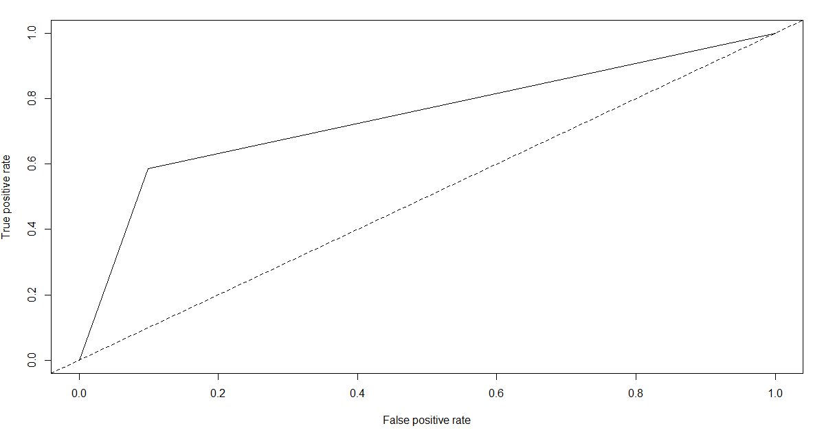
performance(pred.rf.roc,"auc")@y.values

# [[1]]
# [1] 0.7439506

# 성과분석 - 로지스틱 회귀분석

pred.lg <- predict(lg.model,test[,-2],type="response")
pred.lg <- as.data.frame(pred.lg)
pred.lg$survived <- ifelse(pred.lg$pred<=0.5,pred.lg$survived<-"dead",pred.lg$survived<-"survived")
confusionMatrix(data=as.factor(pred.lg$survived),reference=test[,2],positive="survived")

# Confusion Matrix and Statistics
#
# Reference
# Prediction dead survived
# dead      211       57
# survived   32       93
#
# Accuracy : 0.7735
# 95% CI : (0.7289, 0.814)
# No Information Rate : 0.6183
# P-Value [Acc > NIR] : 3.647e-11
#
# Kappa : 0.5044
#
# Mcnemar's Test P-Value : 0.01096
#
#             Sensitivity : 0.6200
#             Specificity : 0.8683
#          Pos Pred Value : 0.7440
#          Neg Pred Value : 0.7873
#              Prevalence : 0.3817
#          Detection Rate : 0.2366
#    Detection Prevalence : 0.3181
#       Balanced Accuracy : 0.7442
#
#        'Positive' Class : survived


pred.lg$survived<-as.factor(pred.lg$survived)
pred.lg.roc<-prediction(as.numeric(pred.lg$survived),as.numeric(test[,2]))
plot(performance(pred.lg.roc,"tpr","fpr"))
abline(a=0,b=1,lty=2,col="black")
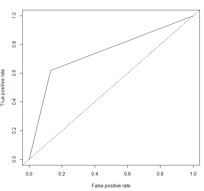
performance(pred.lg.roc,"auc")@y.values


# [[1]]
# [1] 0.7441564